MAPSCI: How does it work?
MAPSCI is a package to estimate cross-interaction parameters of SAFT-\(\gamma\)-Mie using the multipole moments of bead fragments. In this document we will walk through calculations with \(CO_2\) and propane where their parameters are taken from Avendaño 2011 and Dufal 2014, respectively. The multipole moments of these beads are calculated used the DFT method and basis set combination, B3LYP/aug-cc-pVDZ.
Estimation of cross-interaction parameters is achieved in MAPSCI with one of two methods. 1. Analytical Method: Calculation of \(\epsilon_{ij}\) by matching the integral from some lower limit to infinity for the multipole and Mie potentials. 2. Curve-fitting Method: Calculation of \(\epsilon_{ij}\), \(\lambda_{r,ij}\), and \(\lambda_{a,ij}\) by curve fitting the Mie potential to the multipole potential and a consistency constraint using the van der Waals attraction parameter.
Although we are inclined to favor the second method. This tutorial with illustrate why.
Basic Use
First, let’s define the beads library. We excluded the \(CH_2\) bead, because the purpose of this notebook is to simply illustrate the use of MAPSCI. With the parameter library we calculate the cross-interaction parameters with the Analytical and Curve-fitting methods using the default settings. The theory behind this method is temperature dependent and so we must also choose a temperature.
bead_library = {
                "CO2": {
                        'epsilon': 353.55,
                        'sigma': 3.741,
                        'lambdar': 23.0,
                        'lambdaa': 6.66,
                        'Sk': 1.0,
                        'charge': 0.0,
                        'dipole': 0.0,
                        'quadrupole': 4.62033,
                        'ionization_energy': 316.3969563680995,
                        'mass': 0.04401
                       },
               "CH3": {
                       'epsilon': 256.77,
                       'sigma': 4.0773,
                       'lambdar': 15.05,
                       'lambdaa': 6.0,
                       'Sk': 0.57255,
                       'charge': -0.03278,
                       'dipole': 0.068168573,
                       'quadrupole': 0.060537996,
                       'ionization_energy': 254.80129735161324,
                       'mass': 0.01503
                      }
               }
keys = list(bead_library.keys())
import mapsci
temperature = 273
cross_fit, summary_fit = mapsci.extended_combining_rules_fitting(bead_library, temperature)
cross_anal, summary_anal = mapsci.extended_combining_rules_analytical(bead_library, temperature)

print("Parameters from Curve-fitting Method\n\t", cross_fit,"\n")
print("Parameters from Analytical Method\n\t", cross_anal)
Parameters from Curve-fitting Method
     {'CO2': {'CH3': {'epsilon': 274.0094524271247, 'lambdar': 18.705087724553824, 'lambdaa': 6.021868741514751}}}

Parameters from Analytical Method
     {'CO2': {'CH3': {'epsilon': 284.79308252159484}}}
Now let’s compare the multipole potential to the Mie potential from the standard SAFT combining rules and the two parameter sets from our estimation methods.
import matplotlib.pyplot as plt
plt.figure(figsize=(12,6))

# Plot multipole potential
mapsci.plot_multipole_potential_from_dict(bead_library[keys[0]],
                                          bead_library[keys[1]],
                                          temperature=temperature,
                                          plot_terms=False,
                                          plot_opts={"linewidth": 2},
                                          show=False)
# Plot mie potential with SAFT combining rules
mapsci.plot_attractive_mie_potential_from_dict(bead_library[keys[0]],
                                               bead_library[keys[1]],
                                               beadAB={"epsilon": summary_anal[keys[0]][keys[1]]["epsilon_saft"]},
                                               temperature=temperature,
                                               plot_opts={"label": "SAFT",
                                                          "linestyle":"--",
                                                          "linewidth": 2},
                                               show=False)
# Plot mie potential with Analytical method
mapsci.plot_attractive_mie_potential_from_dict(bead_library[keys[0]],
                                               bead_library[keys[1]],
                                               beadAB=cross_anal[keys[0]][keys[1]],
                                               temperature=temperature,
                                               plot_opts={"label": "Analytical",
                                                          "linestyle":":",
                                                          "linewidth": 2},
                                               show=False)
# Plot mie potential with Curve-fitting method
beadAB = mapsci.mie_combining_rules(bead_library[keys[0]],bead_library[keys[1]])
beadAB.update(cross_fit[keys[0]][keys[1]])
mapsci.plot_attractive_mie_potential_from_dict(bead_library[keys[0]],
                                               bead_library[keys[1]],
                                               beadAB=beadAB,
                                               temperature=temperature,
                                               plot_opts={"label": "Curve Fit",
                                                          "linestyle":":",
                                                          "linewidth": 2},
                                               show=False)
plt.legend(loc="best")
plt.xlim((4.25,5.5))
plt.show()

In the plot we see that the traditional SAFT combining rules produce a Mie potential that deviates the most from the multipole potential. The Analytical method of predicting the energy parameter using multipole moments improves the estimation, although the Curve-fitting is much closer.
Next let’s look at the components of the multipole moment that contribute to this fit.
plt.figure(figsize=(12,6))
plt.title("$CO_2-CH_3$ Multipole Potential Contributions")
# Plot multipole potential
mapsci.plot_multipole_potential_from_dict(bead_library[keys[0]],
                                          bead_library[keys[1]],
                                          temperature=temperature,
                                          plot_terms=True,
                                          plot_opts={"linewidth": 2},
                                          show=False)
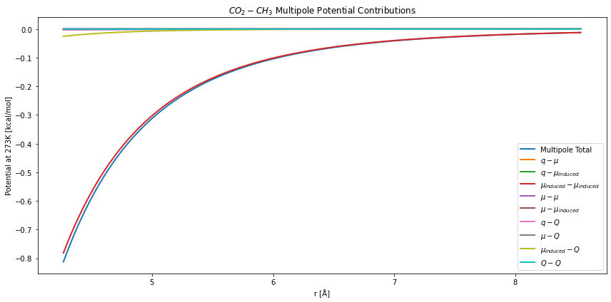
Here we see the largest component is the induced-dipole/induced-dipole interaction. The second largest component is the interactions between dipole and quadrupole moments. In this method the induced-dipole interaction uses the polarizability, which was fit to the provided self-interaction Mie potential.
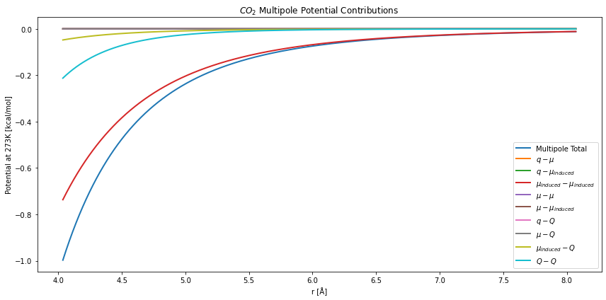
\(CO_2\) has a strong quadrupole moment, but is dominated by the induced-dipole interactions. As seen here:
plt.figure(figsize=(12,6))
plt.title("$CO_2$ Multipole Potential Contributions")
# Plot multipole potential
mapsci.plot_multipole_potential_from_dict(bead_library[keys[0]],
                                          bead_library[keys[0]],
                                          temperature=temperature,
                                          plot_terms=True,
                                          plot_opts={"linewidth": 2},
                                          show=False)
Choosing the Bounds
The results we’ve achieved with our default parameters are encouraging, but how did we choose them? Recall that each method relies on restricting the range of density values. For the Analytical method, each potential is integrated from a minimum bound of integration to infinity. Here we will focus on the Curve-fitting method, which involves defining the lower and upper bound for curve fitting. Setting these bounds will dictate the Mie potential attractive exponent, as the various multipole moments vary in their dependence on distance between beads. For interactions between dipole and induced-dipole moments there is a dependence of \(r^{-6}\). Interactions with these and quadrupole moments follows a dependence of \(r^{-8}\) and with charges the dependence is \(r^{-4}\). At short distances this the total multipole potential will be dominated by \(r^{-6}\) and at longer distances by \(r^{-4}\).
In response to this let’s first take a look at the Mie potential. It is comprised of a repulsive and an attractive potential, although in this work we focus on comparing the multipole potential to the attractive Mie potential.
rmin = mapsci.mie_potential_minimum(beadAB)
r = mapsci.calc_distance_array(beadAB, max_factor=2, lower_bound="sigma")
phi_attractive = mapsci.calc_mie_attractive_potential(r, beadAB)
phi_repulsive = mapsci.calc_mie_repulsive_potential(r, beadAB)

plt.figure(figsize=(12,6))
plt.title("$CO_2$ Mie potential")
plt.plot([r[0],r[-1]],[0,0],"k",linewidth=1)
plt.plot(r,phi_attractive,label="Attractive")
plt.plot(r,phi_repulsive,label="Repulsive")
plt.plot(r,phi_repulsive+phi_attractive,label="Total")
plt.plot([rmin,rmin],
         [min(phi_attractive), max(phi_repulsive)],
         label="Potential Minimum")
plt.plot([beadAB["sigma"],beadAB["sigma"]],
         [min(phi_attractive), max(phi_repulsive)],
         label="$\sigma_{AB}$")
plt.xlabel("$r [\AA]$")
plt.ylabel("Potential at {}K [kcal/mol]".format(temperature))
plt.legend(loc="best")
<matplotlib.legend.Legend at 0x10eeea1d0>
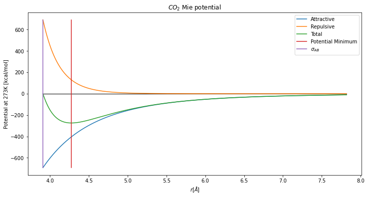
Two natural choices for the Mie potential are (1) the size parameter for the mixed interaction, \(\sigma_{AB}\) and (2) the minimum of the Mie potential. However, notice that the repulsive potential decays faster than the attractive potential. Thus, a third option is a “tolerance” of the ratio of the repulsive term over the attractive term. Since the attractive potential begins dominating the behavior of the Mie potential at \(r_{min}\), our default is to start there.
The maximum density is defined to be a multiple of the lower bound, \(max\_factor\). As discussed previously, the potential shifts its exponential behavior as distance increases. It follows then, that if \(max\_factor\) is too large, then the crucial behavior close to the potential well won’t be represented correctly. Yet, if the range in too small, then the behavior at long distances isn’t captured. We can compare each of these situations by calculating the integral from the lower limit to infinity. We then plot the difference between the integral of the attractive Mie potential with the multipole moment.
mapsci.plot_mie_multipole_integral_difference(bead_library[keys[0]],
                                              bead_library[keys[1]],
                                              temperature,
                                              show=False)
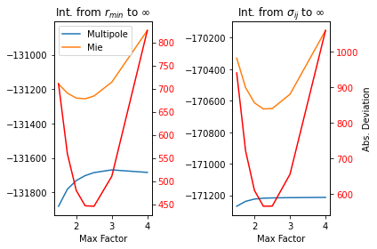
Notice that despite the lower bound (i.e. \(\sigma_{AB}\) or \(r_{min}\)) the least error between the potentials is achieved with a \(max\_factor\) just over two. In addition, the gap is smallest for \(r_{min}\). Hence, our default fitting rangs is from \(r_{min}\) to \(2r_{min}\).